Oracle BI Apps Series - ETL Component Architecture and Functions

This is in continuation to the Oracle BI Apps Series. The first of the posts is BI Applications Architecture

In this post, I want to have a closer look on the ETL architecture of Oracle BI Applications 7.9.6.

Here is a diagram depicting the same -

Next post is about finding various mappings in Informatica and checking how they work..

Hope this helps..

Oracle BI Apps Series - Oracle BI Applications Architecture

Oracle Business Intelligence Architecture Diagram -

I thought its good idea to make a diagram describing various components of BI Apps. Following diagram gives high level architecture of Oracle BI Apps. This is based on my knowledge of 7.9.6 release -

Hope it helps..

OBIEE 11g integration with Microsoft Analysis Services Cubes - Leveraging Statistical capabilities of Analysis Services

OBIEE 11g integration with Microsoft Analysis Services Cubes - Leveraging Statistical capabilities of Analysis Services -

How to use Cube Hierarchies and Statistical Functions together:


As we know, Microsoft Analysis Services has OLAP engine with strong statistical capabilities. Following figure shows the statistical functions available from Microsoft Analysis Services.

I got a question from my client - whether to use OBIEE engine for statistical analysis or do it via pushing to cube by way of MDX.

For those of you, who came directly to this post, some of my last posts discuss about pushing calculations to cube and it may be worth reading those posts.
I checked some statistical functions in OBIEE (I am still checking this), compared it to database functions, and came to know that OBIEE calculates them the same way as Oracle Database does. But my main concern was using the hierarchies with statistical functions.

Although, I was able to calculate statistical functions along with hierarchies by writing SQL code, it seems quite difficult to model in OBIEE.

Analysis Services has strong statistical capabilities and I tend to use them for my purpose.

Let's start with MEDIAN.

'Median' is an important measure of central tendency of a sample. I know that, everybody is aware about the definition of median, but just for the sake of completeness, I want to summarize it here:

Definition - Median:

The median is the value of the middle item of a set of items that has been sorted into ascending or descending order.
In an odd-numbered sample of n items, the median occupies the (n+1)/2 position. In an even-numbered sample, we define the median as the mean of the values of items occupying the n/2 and (n+2)/2 positions (the two middle terms).

In this post, I want to show the way to calculate median over a data set (product dimension and sales amounts) and how the other dimensions will affect the calculation.
The cube is as shown below:

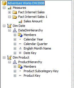
The cube has two dimensions -

1. Dim Date
2. Dim Product

Each of these dimensions has one hierarchy which can be seen in the adjacent figure.

The measure used to calculate the median is 'Sales Amount'.









Following is the logical model diagram, in OBIEE:

As you can see, its very simple model. Its just the cube measures, product and date dimensions.

The challenge here is to pass the cube hierarchies through the logical layer of OBIEE, and preserve the drill down for these hierarchies and statistical calculations at the same time.

This can be achieved by Fixing the currentmembers in those dimensions which we want to appear in the report and calculating the statistical function on the dimension we want.

In simple terms, we can start with fixing our currentmember to e.g. 'August 2002' and then calculate the median of Sales Amount over Product dimension. So I ask cube to first fix the currentmember to 'August 2002'. Then pick a member from Product dimension. And for the member which is picked from Product dimension, give me the median over all its children.

This can be achieved by the following expression:

evaluate_aggr('median({[Dim Date.DateDimHierarchy].currentmember* [Dim Product.ProductHierarchy].children}, [Measures].[Sales Amount])' as double)

You are free to use this in the formula tab of Answers, or in RPD.

Now let's have a look on the analysis - How our drill down and statistics work together:

I made a simple analysis with putting a filter on Month column, and including Month, Product, and other metrics in the report.

Following is the figure which shows the formula in the answers:

Following is the results:

The above figure shows data at the lowermost level. You can see the sales amount for each product.

The median over this sample should be (20714.20 + 18642.78)/2.

This can be seen in the figure below:

Now the median over product subcategory 1 and 2 should be (412207.41 + 133794.06)/2. Since we'll always calculate median over the sales amount at a particular level. There is not much use of calculating a median over a median.

This can be seen in the next figure:

So we saw, how we can preserve hierarchical relationships and statistical calculations together in the same analysis.

This is a simple scenario. Even complex situations can be achieved by using this approach.
Calculation of standard deviation is similar to median with the help of following expression:

evaluate_aggr('stddev({[Dim Date.DateDimHierarchy].currentmember* [Dim Product.ProductHierarchy].children}, [Measures].[Sales Amount])' as double)
Standard Deviation tells us - how much variation or "dispersion" there is from the "average", which is again very important measure to have an insight into the data.

Hope this post will be useful to readers. Comments appreciated. Thanks.

OBIEE 11g and Multidimensional Data Sources - How to achieve Custom Aggregations (CASE STATEMENTS)

I have come across a very interesting scenario for handling the Custom Aggregations in OBIEE against Multidimensional Sources.

I want to start this post with a simple view of a MSAS cube in Microsoft Business Intelligence Development Studio. My aim is to show different types of aggregations available, while building the cube.

Whenever a cube is built in MSAS, an aggregation rule (AggregateFunction) is assigned to the measure. This can be seen in the following figure:

The figure shows the structure of a very simple MSAS cube. The aggregation rule in this example is 'DistinctCount'.

This measure is actually a Customer Key column in the Fact Table in the Data Warehouse.

Different technologies have different ways to aggregate data. As you are already aware, that in OBIEE we put aggregation rule over a measure in the fact table (we can put different aggregation rules for different dimensions in OBIEE). Hyperion Essbase has a completely different way to handle the aggregations. It has capability to assign the aggregation operator to each member of its dimension. The comparison of aggregation strategies among various tools is the idea of a different post.


















For those, who want to know the other possible aggregation rules available in MSAS, the following screenshot may be helpful:

The most common aggregation rule we encounter in our day to day interactions with BI and DW systems is 'Sum', which is pretty straightforward to handle.

Other frequently used Aggregation rules are Average, Min, Max etc.

Once the cube is built in the Microsoft BI Development Studio, its deployed, and then processed.

For OBIEE perspective, we'll not go to depth of these terms and their effects, but once a cube gets processed successfully, it contains the measure value for each of the possible combinations of its dimension members.

The best way to explore a cube, is either through Microsoft Excel, or through Microsoft SQL Server Management Studio, where you can drag and drop hierarchies, levels, and measures easily over the canvas.

If a measure in the cube is having aggregation rule 'Sum', then its perfectly possible to take day/month level data (e.g. product sales for day/month) in OBIEE, and aggregate rest of the levels e.g. Quarter/Year etc in OBIEE by putting an aggregation rule in fact measure.

But for measures like 'Customer Count' data needs to be provided by the cube. Its not possible for OBIEE to have day/month level data for 'Customer Count' and aggregate it to Quarter, year level, without having customer keys.


This is the reason for having 'External Aggregation' rule in OBIEE for COUNT DISTINCT measures. This is described in this post. I discussed the function shipping abilities too in the same post.

Now let's discuss the Custom Aggregations:

There are many types of Custom Aggregations. What I am going to discuss here is a special case i.e. CASE STATEMENTS.

Following is my Data Set:

The Customer Count for January 2003 is 244.
January 2004 is 1777.











and the Customer Count for January 2003 AND January 2004 is 1973 (due to overlapping customers), as can be seen below.

The job is to model this in OBIEE such that, I have two columns in the Report -  Column1. CASE WHEN Month_name IN ('January 2003', 'January 2004') THEN 'January 2003/4' ELSE Month_name END
Column2. Customer Count.


This is pretty straightforward. Here are the steps:
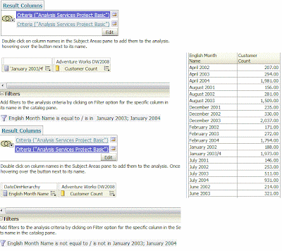
Step 1. Make an analysis with Month Name and customer count. Put a Filter on Month Name so that it contains only January 2003 and January 2004. Use Edit formula of Month Name column so that it contains a literal 'January 2003/4'
Step 2. Combined this analysis with similar analysis with different filter i.e. excluding January 2003 and January 2004

Here are the analyses and the results:

Results as expected.

Now the same question with a twist - I need to see Customer Count for the whole year 2003 and Month January 2004 as in One row, and rest of the months as usual.

So I need two columns in the report -
Column1 - CASE WHEN (Month Name = 'January 2004' AND Year = 2003) THEN 'Custom Selection' ELSE Month Name END
Column2 - Customer Count

Here is what exists in the cube (This is when I explored the cube from Microsoft Studio):

If I follow the same approach of putting filters, then its not going to give me any data, as shown below:

 The reason its not giving me any data lies in MDX it generates, but at the moment I don't want to explore that way.














What I'm going to do is to Call MDX AGGREGATE function from OBIEE and pass it the parameters as below:

What I have done is to pass these two dimension members i.e. year 2003 and Month January 2004 to MDX AGGREGATE function, with a measure.









We need to set the aggregation rule over this column to 'Evaluate_Aggr' as below:

Otherwise its not going to pass the repository consistency check.









I created the report, and got the results as expected:

We can combine this with a similar request to show other months. It seems to work the way expected. We can even put other dimensions and measures in the analysis and it should work fine.

I hope this post would be useful to the readers. Comments appreciated. Thanks.

OBIEE 11g integration with Microsoft Analysis Services Cubes - Aggregation Rules and Count Distinct

As we know, OBIEE has great federation capabilities, and they are used to federate multiple environments. Organizations sometimes have a mix of disparate systems e.g. Oracle Databases, SQL Servers, MSAS/Essbase Cubes etc, and it is always expected to federate them all for a unified view of the data.

Federation itself is a different topic and conformed dimensions play a vital role over there. Its the idea of a different post. For this post, I want to have a look on the Microsoft Analysis Services cubes' inbuilt aggregations and how to leverage it.

My environment consists of:
1. OBIEE 11g
2. Microsoft Analysis Services 2008

I used AdventureWorks2008 database, which is a sample database for SQL Server/MSAS. I have built a basic cube with two dimensions and a measure for 'Customer Count'. The aggregation rule to build this measure in MSAS is 'DistinctCount'. It is shown below:

As we can see in the above figure, the measure 'Customer Count' is of the nature of  'COUNT DISTINCT' and so is non-additive. The lowest level for which data is stored in the cube is Date.

I imported the cube in the physical layer of the RPD. The measure 'Customer Count' is available with both the hierarchies. Following is the property of this physical cube column:

As we can see, the Aggregation Rule set in the physical layer of RPD is 'External Aggregation'.
'External Aggregation' pushes all the aggregations to be performed to the cube, and doesn't aggregate data in OBIEE. Sometimes there are doubts for this Aggregation Rule strategy, whether to set it to match with the cube (in this case COUNT DISTINCT) or leave it to External Aggregation etc...

The rule of thumb is - Push as much as possible to the Cube, especially non-additive or semi-additive measures. The cubes (either MSAS or Essbase) are created with aggregated data. The technology behind these products allows them to address a particular cell of the cube quickly.

For non-additive measures, we can aggregate data in OBIEE only when we have the lowest level of details available. In this example it would be the customer account numbers, which are eventually not available. So putting a COUNT DISTINCT over this measure in OBIEE would do nothing, but will return me COUNT DISTINCT (data in the cells). And this would result in erroneous data.

So I'll leave the aggregation rule to 'External Aggregation' in physical as well as logical layer of OBIEE.

I tried to create an analysis with Year and the Customer Count, which seems absolutely fine to me:

So we can develop the reports with this approach, we can drill down in hierarchies etc. But its bit tricky to use the CASE STATEMENTS when we use 'External Aggregation' as the aggregation rule in OBIEE.

CASE STATEMENTS are not yet function shipped to back end Cubes in MSAS.

This means that in any of the report if I'll try to aggregate data (CASE STATEMENTS belong to Custom Aggregations class) explicitly, then I am going to get function ship error.

Below is a snippet of this error -

//

State: HY000. Code: 10058. [NQODBC] [SQL_STATE: HY000] [nQSError: 10058] A general error has occurred. [nQSError: 43113] Message returned from OBIS. [nQSError: 43119] Query Failed: [nQSError: 42015] Cannot function ship the following expression: AggrExternal(Adventure Works DW2008.Customer Count by [ case when Adventure Works DW2008.English Month Name in ([ 'February 2004', 'January 2004', 'March 2004'] ) then 'Com months' else Adventure Works DW2008.English Month Name end ] ). (HY000)

//

So what I tried to do is to combine Jan, Feb, Mar 2004 in a case statement and to pass it to the Cube. OBIEE is unable to function ship this to the MSAS cube. Future releases of OBIEE are expected to address the custom aggregations, but till then there is a workaround.

How to achieve the custom aggregations by passing MDX functions to MSAS is the topic of my next post. Thanks.


The next post can be found here.

OBIEE 11g Time Series Analysis against Microsoft Analysis Services Cube

Recently, I got an opportunity to explore the OBIEE integration with Microsoft Analysis Services. I came across some advantages and some limitations too. In our environment, we are using OBIEE 11g, which supports time-series analysis against Cubes. Even in case of OBIEE 10g, the functionality was supported after applying a patch from Oracle. So in this post, we'll have a look on two ways to achieve time series analysis against Cubes -

1. By using OBIEE functions (I'll use Ago for this post).
2. By using MDX lag function (Passing this from OBIEE's EVALUATE_AGGR).

Let's start with OBIEE AGO function -

I created a test cube, with just one dimension i.e. time, and some measures by using Microsoft BI Development Studio. The cube is shown below:


Figure 1 - Cube

I imported the cube in the Physical layer of the RPD, and then simply dragged it to the logical layer. In the logical layer I created a derived measure by using AGO function. The name of this derived column is 'Amount Previous Period':

Figure 2 - Logical Column for AGO

Although, the syntax for using Ago is -  Ago(<<Measure>>, <<Level>>, <<Number of Periods>>), but it can be used without specifying the <<Level>>, if we want to make it dynamic. In this way, it can be used with all the levels in the time dimension.

Now I want to create a simple analysis with just three columns - Year, Amount, and Amount Previous Period.

As you can see, its working as expected. Same analysis, but with Month (which is a chronological key in the Business Model) will look like below:

Below is the MDX which got generated for the above analyses:



//
With 


    set [Dim Date Test.Hierarchy3]  as '{[Dim Date Test.Hierarchy].[Monthseq].members}'
set [Axis1Set] as '{[Dim Date Test.Hierarchy3]}'
  
  member [Measures].[MS2] as 'SUM({ParallelPeriod([Dim Date Test.Hierarchy].[Monthseq], 1,[Dim Date Test.Hierarchy].currentmember)},[Measures].[Amount])'
  
select 
  {[Measures].[Amount],[Measures].[MS2]} on columns,
  NONEMPTY({[Axis1Set]},{[Measures].[Amount],[Measures].[MS2]}) on rows 
from 
  [Test]

//

As we can see, in the background its 'ParallelPeiod' which is doing the calculation for OBIEE.


Now let's have a look at the MDX lag function, and how to pass it from OBIEE using EVALUATE_AGGR:


Below is the logical column for this:

The hierarchy which is passed to  EVALUATE_AGGR, can be picked from the physical layer of the RPD. Currentmember makes it dynamic across levels. lag(1) takes it one period back.

Below is the same analysis for year, amount, and amount for prev period - lag

As we can see, its exactly the same result. Below is the MDX which got generated this time:

//

With 


    set [Dim Date Test.Hierarchy2]  as '{[Dim Date Test.Hierarchy].[Calendar Year].members}'
set [Axis1Set] as '{[Dim Date Test.Hierarchy2]}'
  
  member [Measures].[MS2] as '([Dim Date Test.Hierarchy].currentmember.lag(1), [Measures].[Amount])'
  
select 
  {[Measures].[Amount],[Measures].[MS2]} on columns,
   NONEMPTY({[Axis1Set]},{[Measures].[Amount],[Measures].[MS2]}) on rows 
from 
  [Test]
//

As we can see in the MDX, this time the function used is lag.

Both of these approaches seem equivalent as they tend to the same results. In case of using 'Ago' in OBIEE, we need a chronological key to be exposed from the cube, which may not always be the case in some environments. I prefer the way to do it in MDX since we have much control over it.

Hope this post will be useful to the readers. In the next post, I am planning to write about aggregations in Cube/OBIEE. The post can be found here. Thanks.